excel拖动排列步骤如下:1.我在EXCEL中输入以下数字,如图:2.现在我要想复制“1”,则拖动单元格A1,但此该你会发现,在下拖动下方有个方框,如图:3.上步出现的情况便是以顺序的方式出现,但你只需要点动那个右下方的方框,选择“复制单元格”即可......
excel 柱形图教程制作详细步骤及技巧
Excel教程
2021-09-30 15:14:46
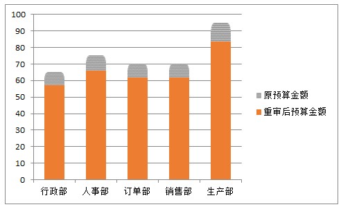
【效果图】如下↓

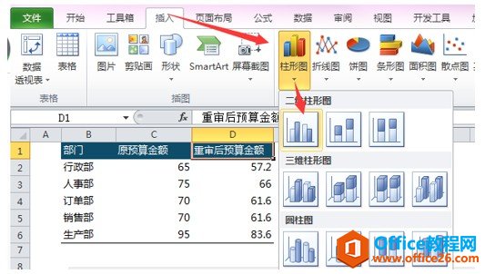
Excel柱形图教程制作详细步骤如下: 1. 选中B2:D6区域【插入】-【二维柱形图】-【簇状柱形图】,或者选中区域直接按ALT+F1快速插入图表
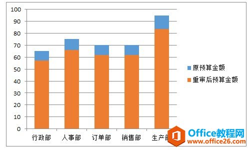
 2. 选中蓝色柱子,右键-【设置数据系列格式】-【系列选项】-【系列重叠】-100%,【系列间距】106%
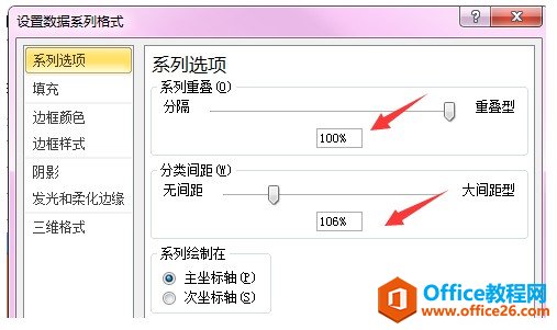
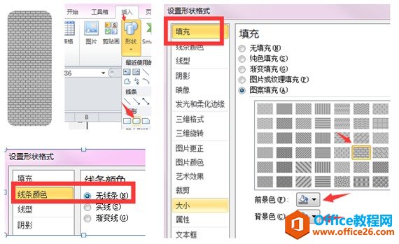
3. 【插入】-【形状】-【圆角矩形】,右键【设置开关格式】-【线条颜色】-无,【填充】-【图案填充】,设置前景色与后景色的颜色。
4. 复制设置好的形状,按CTRL+C,然后选中蓝色柱子,按CTRL+V,效果如下:
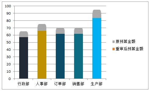
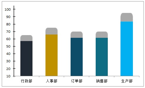
 5. 单击一次橙色柱子,再单击一次行政部的橙色柱子,右键-【设置数据点格式】-【填充】-【纯色填充】-选择一个颜色,同理设置其他几个部门的橙色柱子。
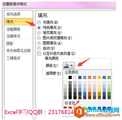
6. 选中网格线-按DEL键删除。选中图例删除。
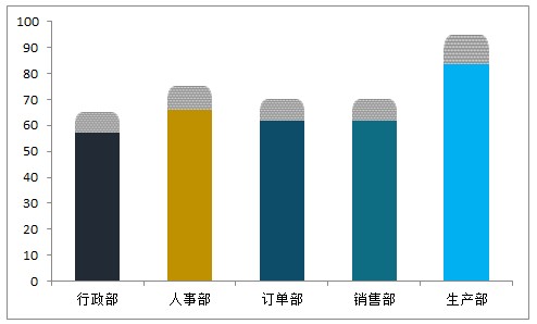
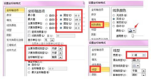
7. 选中纵坐标轴,右键-【设置坐标轴格式】-最小值设为10,最大值设为105,主要与次要刻度单位都设置成10.【主要刻度线类型】选内部,【次要刻度线类型】选外部。坐标轴标签使用默认选项轴旁即可。
 8. 选中横坐标轴,右键-【设置坐标轴格式】-【坐标轴选项】-主要刻度类型-无,次要刻度类型-外部。【线条颜色】-灰色,线型-2磅。
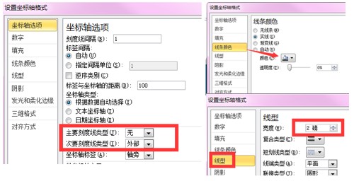
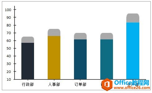
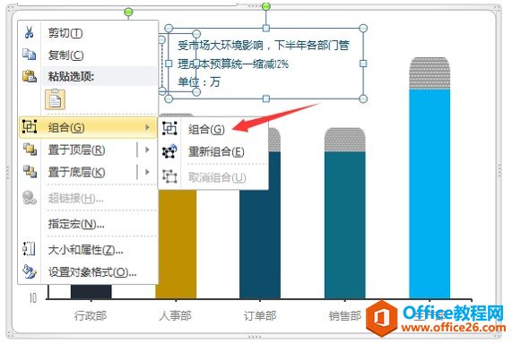
9. 插入一根竖线及两个文本框,文本框内写上对应内容。按住CTRL键同时选中直线,文本框与图表右键组合,组合后它们就成一个整体了。
10. 选中图表区,右键-【设置图表区格式】-【填充】-纯色填充:灰色;【边框颜色】-无线条;【阴影】外部第一个。选中矮柱子系列,右键-【添加数据标签】,设置【数据标签格式】-标签位置-轴内侧。

OK,完工。小编需要提醒一下,我们做图时不仅要有颜值,更要修炼内功,内外兼修方是上上之策。如何去解说一份图表,如何让图表来帮助我们看清数据,以及利用图表来支撑我们的数据观点更加重要。因为我们毕竟不是玩图,元芳,你怎么看?
标签: excel柱形图教程制作
相关文章